miniTE Technical Report: Stable and Efficient Reinforcement Learning with Native NVFP4

On this page

• TL;DR
• Abstract
• 1. Introduction
• 2. Why Native NVFP4 RL Becomes Unstable
• 2.1 Failure Develops During Training
• 2.2 Quantization Error, Conversion Error, and Execution Mismatch
• 2.3 Activation Precision, Scaling Granularity, and the KV Cache
• 2.4 Mismatch Must Be Interpreted Alongside Update Direction
• 2.5 Averages Can Hide Local Risk
• 3. TRIAGE: Direction-Aware Stabilization of Native NVFP4 RL
• 3.1 Mechanism
• 3.2 Stability and Task Performance
• 3.3 Complementary Algorithm and Engineering Tracks
• 4. miniTE: Aligning Numerical Execution and Optimizing Low-Precision Compute
• 4.1 Controlling Numerical Differences and Execution Cost
• 4.2 Layered Interfaces and Transformer Engine Integration
• 4.3 Precision Recipes and Selective Quantization
• 4.4 Numerical Monitoring, Profiling, and Alignment Diagnostics
• 4.5 Train–Inference Alignment and Deterministic Execution (Deterministic Mode)
• 5. Joint NVFP4 Implementation and Optimization with Transformer Engine
• 5.1 Numerical and Implementation Choices for Per-Token Scaling
• 5.2 Contiguous Layouts and Grouped GEMM Invocation
• 5.3 Computing amax Where Data Are Produced
• 5.4 Kernel Optimizations and Their Scope
• 5.5 How Joint Testing Informs Implementation Choices
• 5.6 Exploring Single-Pass Fusion
• 6. Evaluation: Numerical Correctness, Learning, and Execution Efficiency
• 6.1 Setup and Measurement Scope
• 6.2 Correctness and Learning Behavior
• 6.3 Complete Learner Updates: Do Local Changes Reduce Update Cost?
• 6.4 Modules: Faster Forward Does Not Necessarily Mean Faster F+B
• 6.5 Rollout and Online RL: System Gains and Remaining Costs
• 6.6 What the Experiments Establish
• 7. Using and Extending miniTE
• 7.1 Integrating Existing Models through Linear Interfaces
• 7.2 Explicit Recipes and Precision Boundaries
• 7.3 Diagnostics as Part of Extension Development
• 8. Discussion: From Numerical Alignment to End-to-End Learning
• 8.1 Weight Updates and Synchronization Remain a Bottleneck
• 8.2 Why Does Low Precision Remain Sensitive After Operator Alignment?
• 8.3 Optimize Updates and Final Learning Outcomes
• Appendix A. Experimental Setup and Statistics
• A.1 Supplementary Algorithm and Training Materials
• A.2 Supplementary Long-Run RL and Checkpoint Evaluation
• A.3 Fixed-Text miniTE Learner Tests
• A.4 Module, Serving, and RL Stage Timing
• Appendix B. TRIAGE Method Conventions
• References

TL;DR

• Problem and diagnosis · Native NVFP4 RL can become unstable late in training. We examine quantization, activation scaling, KV caches, and execution paths, then study how their errors affect updates.
• Algorithm & engineering · TRIAGE controls residual mismatch risk through update direction. miniTE reduces numerical execution differences and optimizes low-precision computation. We evaluate them separately.
• Measured gains · On 8×B300, miniTE with BF16 backward achieves approximately 1.33–1.37× BF16 speed for complete learner updates. A separate fixed-output serving test reaches approximately 1.64× throughput.
• Limits and open questions · In the reported online RL run, weight conversion and synchronization offset sampling gains. The practical miniTE checkpoint also remains below BF16 on the five-task average. Matching operators and obtaining a small gap do not guarantee BF16-level learning; error tolerance, update rules, and final outcomes need further study.

Abstract

Native NVFP4 reinforcement learning must remain stable under quantization and execution error while delivering practical efficiency gains. We investigate late-training instability by examining quantization formats, activation scaling, KV-cache precision, and framework differences that affect policy probabilities. TRIAGE addresses residual mismatch by adjusting updates in high-risk segments according to the mismatch and update directions, improving stability and task performance. miniTE separates quantization policy, linear layers, and compute backends, providing precision configuration, alignment checks, and performance analysis. Joint work on Transformer Engine’s per-token NVFP4 path uses contiguous layouts, device-side metadata, amax (maximum absolute value) reuse, grouped GEMM, and fusion to reduce preparation and dispatch overhead. On 8×B300, both miniTE paths with BF16 backward achieve approximately 1.33–1.37× paired speedups over BF16 for complete learner updates. A separate fixed-output serving test reaches approximately 1.64× BF16 throughput. These learning and system results come from separate configurations; lower mismatch and faster local computation do not yet establish BF16-level learning or an end-to-end RL speedup.

1. Introduction

Reinforcement learning for large language models repeatedly performs rollouts, policy-probability recomputation, gradient updates, and weight synchronization. Long responses increase the token volume for both generation and training, making low-precision computation valuable. Blackwell supports native NVFP4 matrix multiplication, and prior pretraining work has demonstrated low-bit training with scaling, mixed precision, and suitable rounding strategies [1]. An RL loop must additionally connect the numerical implementations used by the training and inference frameworks.

Our early NVFP4 runs improved reward initially but later developed abnormal entropy, growing training–sampling log-probability gaps, and declining reward. Quantization error, checkpoint conversion, activation scaling, KV-cache precision, and operator execution on both sides affected the outcome. Replacing a single quantization operator, or confirming that both sides used NVFP4, did not resolve all of these issues.

We first describe the failures, then use controlled experiments to identify and locate their causes. This leads to complementary algorithmic and engineering tracks. TRIAGE changes the update rule to control the effect of residual mismatch on learning. miniTE acts on numerical execution, reducing avoidable differences while turning low-precision computation into practical efficiency gains.

In a large training framework, changing scale granularity or a GEMM backend can require changes to layer wrappers, grouped layouts, communication, and autograd. miniTE separates quantization policy from these shared functions, allowing developers to replace a compute path within an existing training workflow and then evaluate its numerical correctness, learning behavior, and runtime cost.

Section 2 traces native NVFP4 RL failures and their diagnosis. Section 3 presents TRIAGE and its results. Sections 4–7 describe miniTE, implementation optimizations, experiments, and usage. We report algorithmic outcomes and system performance separately, with the configuration for each experiment.

2. Why Native NVFP4 RL Becomes Unstable

2.1 Failure Develops During Training

We run GRPO on DAPO mathematics tasks with Qwen3-4B and Qwen3-30B-A3B [4,5,6]. In early native NVFP4 runs, reward increased normally before training deteriorated. In the trajectories analyzed by TRIAGE, the 4B model became unstable after approximately 300 steps, while mismatch in the 30B model began growing rapidly after approximately 700 steps. Diagnosing this process requires measurements over training time rather than a single initial error value or a short loss curve.

We track reward, entropy, the training–sampling log-probability gap, and downstream task scores. For token ttt in response iii, define δi,t=log⁡πl(yi,t∣xi,yi,<t)−log⁡πs(yi,t∣xi,yi,<t)\delta_{i,t}=\log\pi_{\mathrm l}(y_{i,t}\mid x_i,y_{i,<t})-\log\pi_{\mathrm s}(y_{i,t}\mid x_i,y_{i,<t})δi,t​=logπl​(yi,t​∣xi​,yi,<t​)−logπs​(yi,t​∣xi​,yi,<t​). Here xix_ixi​ is the prompt, yi,ty_{i,t}yi,t​ is the current token, and yi,<ty_{i,<t}yi,<t​ is its generated prefix. The learner and sampler assign conditional probabilities πl\pi_{\mathrm l}πl​ and πs\pi_{\mathrm s}πs​; log⁡\loglog denotes the natural logarithm. A negative gap means the learner assigns a lower probability, and a positive gap means it assigns a higher one. Mean absolute gap averages ∣δi,t∣|\delta_{i,t}|∣δi,t​∣ over the tokens being evaluated.

2.2 Quantization Error, Conversion Error, and Execution Mismatch

Quantization error compares low-precision computation with a higher-precision reference. Training–sampling mismatch compares the actual executions of the learner and sampler. Checkpoint conversion and inference-backend adaptation can introduce additional error. Before integrating RL, we therefore compare BF16 inference, online NVFP4 quantization, and inference using offline-converted NVFP4 weights.

NVFP4 represents quantized values in E2M1: E and M give the exponent and mantissa bit counts, with one additional sign bit. Decoding gives x^=q,sb,sg\hat x=q,s_b,s_gx^=q,sb​,sg​, where qqq is the E2M1 value, sbs_bsb​ is an E4M3 block scale shared by 16 elements, and sgs_gsg​ is an FP32 outer scale. The recipe determines whether the outer scale is computed per tensor, per expert, or per row.

E2M1 data occupy 4 bits. Each block of 16 elements shares an E4M3 scale, with an additional outer FP32 scale. Click the payload bits and change the scales to inspect finite values and reconstruction. The example scales are representable values.

Open interactive figure: inspect values, switch configurations, download SVG / CSV

A Qwen3-0.6B NVFP4 pretraining checkpoint initially suffered severe performance degradation because its fused QKV structure was handled incorrectly. After the fix, mean Lambda accuracy was approximately 0.3043 for BF16, 0.3056 for one-dimensional quantization, and 0.3109 for two-dimensional block-scaled quantization. Conversion and structural adaptation must therefore be checked before attributing such a failure to the FP4 format.

For Qwen3-4B, online quantization reduced Lambda-base and Math23K scores by 0.0355 and 0.047 relative to BF16. Offline conversion introduced additional reductions of 0.0089 and 0.019. These comparisons separate the loss from the format and numerical path from the additional loss introduced by conversion and scale handling.

In RL, the two sides can differ substantially even when they use the same format. Early configurations produced the following mean absolute log-probability gaps:

Training / sampling precision	Dense	MoE
BF16／BF16	0.0110	0.0172
NVFP4／NVFP4	0.1142	0.0668
NVFP4／BF16	0.1376	0.0621
BF16／NVFP4	0.1690	0.0747

Table 1. Early training–sampling comparisons. The dense model is Qwen3-4B; the MoE model is Qwen3-30B-A3B. These results locate error sources within this set of configurations.

Replacing offline ModelOpt conversion with online quantization still left a gap of approximately 0.1142 for the dense model. Using the same quantization/GEMM operators on both sides also left residual differences. We therefore expanded the investigation to input organization, scale computation, and operations surrounding quantization.

2.3 Activation Precision, Scaling Granularity, and the KV Cache

With NVFP4 weights fixed, increasing activation precision tests the effect of activation quantization. W and A denote weights and activations; the following numbers give their bit widths, so W4A16 uses 4-bit weights and 16-bit activations:

Weights / activations	Dense gap	MoE gap
W4A16	0.0139	0.0166
W4A8, MXFP8 activations	0.0363	0.0227
W4A4, NVFP4 activations	0.0903	0.0445

Table 2. Activation-precision comparisons using the corresponding unquant inference adaptation paths. This experiment and Table 1 belong to different stages of the investigation and are not a single ablation.

W4A16 brings the gap close to the BF16 reference, identifying activation quantization as an important factor in this configuration. In another fixed configuration, changing the KV cache from FP8 to BF16 reduces the gap from 0.0721 to 0.0583. Sampler-state precision also affects cross-framework agreement.

We next examine the scaling domain. Sampler decoding processes the current token, whereas the learner typically processes a full response at once. If the activation’s outer scale uses tensor-wide amax, the same token can receive different scales depending on the other tokens in its batch. Per-token amax restricts the reduction domain to the current row and removes this dependency.

Let xxx be a reference vector and x^\hat xx^ its decoded approximation, each with nnn elements. Relative L2 error is ∣x^−x∣2/∣x∣2|\hat x-x|_2/|x|_2∣x^−x∣2​/∣x∣2​; signal-to-noise ratio is SNR=20log⁡10(∣x∣2/∣x^−x∣2)\mathrm{SNR}=20\log_{10}(|x|_2/|\hat x-x|_2)SNR=20log10​(∣x∣2​/∣x^−x∣2​), in dB; and mean absolute error is MAE=n−1∑j=1n∣x^j−xj∣\mathrm{MAE}=n^{-1}\sum_{j=1}^{n}|\hat x_j-x_j|MAE=n−1∑j=1n​∣x^j​−xj​∣. The notation ∣⋅∣2|\cdot|_2∣⋅∣2​ denotes the Euclidean norm. Relative error and SNR assume a nonzero reference vector. Lower relative L2 and MAE, or higher SNR, indicate closer reconstruction.

The target token’s 32 inputs remain fixed; the slider changes only another token’s amax in the batch. A finite E2M1/E4M3 codebook with round-to-nearest-even shows block scales, reconstructed values, and relative L2 error. This is a mathematical example rather than a model or GPU measurement; it excludes RHT, SR, FTZ, and padding. The print version shows the constructed inputs and reconstructed values at the default amplitude.

Open interactive figure: inspect values, switch configurations, download SVG / CSV

Scaling granularity does not determine all quantization error. We sweep exponent and mantissa widths on real QKV inputs. With E=2 and E4M3 scales fixed, increasing M from 1 to 4 raises mean SNR from 19.88 dB to 34.96 dB and reduces relative L2 from 0.10140 to 0.01807. Increasing exponent width does not always help and can interact poorly with the scale’s representable range. These simulated formats identify sensitive factors; they are not additional hardware-native NVFP4 formats.

In one configuration, per-token amax changes the initial gap only slightly, from 0.05532 to 0.05501, while later runs show smoother training. This motivates examining error direction, local structure, and its evolution during training rather than relying on the initial average alone.

D1 · Exponent and Mantissa Sweeps: Real QKV Inputs, Simulations, and Initial RL Measurements

Real QKV Inputs: Varying Mantissa Width

Format	SNR E4M3	SNR E8M0	Rel-L2 E4M3	Rel-L2 E8M0
E2M1	19.88	17.11	0.10140	0.13950
E2M2	26.23	23.98	0.04885	0.06322
E2M3	31.19	30.31	0.02767	0.03051
E2M4	34.96	36.41	0.01807	0.01513

Table 2-1. QKV inputs collected from 36 layers during real prefill and single-token generation, summarized across layers. The simulated formats do not imply new hardware support.

Real Inputs: Exponent Range and Scale Range

Data format	SNR with E4M3 (dB)	SNR with E8M0 (dB)
E2M1	19.88	17.11
E3M1	21.50	19.7
E4M1	14.39	19.7
E5M1	0.0 (maximum exceeds E4M3 range)	19.7

Data format	Relative L2 with E4M3	Relative L2 with E8M0
E2M1	0.10140	0.13950
E3M1	0.08478	～0.103
E4M1	0.28937	～0.103
E5M1	0.99698 (maximum exceeds E4M3 range)	～0.103

E3M1/E4M1/E5M1 with E8M0 scales behave similarly over the measured input range. Combining E4M3 scales with a wider data range can create scale-range problems. More exponent bits therefore do not necessarily improve accuracy for these inputs.

Initial RL Gap: Exponent and Mantissa Width

Data format	Initial gap with E4M3
E2M1	0.05800700932741165
E3M1	0.11516289412975311
E4M1	3.412203073501587
E5M1	nan

Data format	Initial gap with E4M3
E2M1	0.05800700932741165
E2M2	0.042353976517915726
E2M3	0.03562581539154053
E2M4	0.031815189868211746

Table 2-2. Recorded initial gaps, including NaN outcomes. These measure initial agreement; long-run training is evaluated separately.

Simulated Inputs and Real-Input Comparisons

Data format	Scale format	MAE	SNR dB
E5M1	E4M3	1.485030	0.00
E4M1	E4M3	0.132963	20.48
E3M1	E4M3	0.127780	20.63
E2M1	E4M3	0.154619	19.62
E5M1	E8M0	0.128281	20.18
E4M1	E8M0	0.128281	20.18
E3M1	E8M0	0.128515	20.18
E2M1	E8M0	0.176643	17.97

Data format	Scale format	MAE	SNR dB
E2M4	E4M3	0.017888	36.91
E2M3	E4M3	0.034627	31.58
E2M2	E4M3	0.070138	26.04
E2M1	E4M3	0.142116	20.17
E2M4	E8M0	0.018970	37.03
E2M3	E8M0	0.038432	30.93
E2M2	E8M0	0.079777	24.93
E2M1	E8M0	0.176643	17.97

Table 2-3. MAE/SNR from two simulated input batches, corresponding to exponent and mantissa sweeps. They separate input-distribution effects from bit-width effects and are distinct from repeated measurements of real QKV means. The complete format summary follows.

Format	Mean SNR	Worst SNR	Mean MAE	Mean relative L2
E2M4 + E8M0	36.41	35.87	0.007954	0.01513
E2M4 + E4M3	34.96	29.58	0.007589	0.01807
E2M3 + E4M3	31.19	28.12	0.014404	0.02767
E2M3 + E8M0	30.31	29.73	0.016283	0.03051
E2M2 + E4M3	26.23	25.03	0.027865	0.04885
E2M2 + E8M0	23.98	23.64	0.034200	0.06322
E3M1 + E4M3	21.50	17.81	0.045411	0.08478
E2M1 + E4M3	19.88	19.53	0.058788	0.10140
E5M1/E4M1/E3M1 + E8M0	~19.7	~19.3	~0.051	~0.103
E2M1 + E8M0	17.11	16.66	0.077184	0.13950
E4M1 + E4M3	14.39	0.71	0.067209	0.28937
E5M1 + E4M3	0.03	0.00	0.577118	0.99698

2.4 Mismatch Must Be Interpreted Alongside Update Direction

Let AiA_iAi​ denote the advantage of response iii, measuring its reward relative to other responses in the same group. The figure abbreviates it as AAA and writes a token’s gap as δ\deltaδ. In GRPO, a positive advantage tends to increase sampled-token probabilities; a negative advantage tends to decrease them. At synchronized weights, the gap reflects execution differences. After learner updates, it also includes parameter changes relative to the fixed sampling policy.

When the learner underestimates a token (δ < 0), a negative-advantage update lowers its probability further and can amplify the local discrepancy; a positive-advantage update tends to reduce it. The roles reverse when the learner overestimates the token (δ > 0).

Intervention therefore needs both gap magnitude and update direction. TRIAGE uses the signs of advantage and gap to identify local risk. This local analysis motivates the algorithm; actual updates also depend on cross-token coupling and the optimizer.

Change the signs of advantage and gap to inspect local amplification or contraction and TRIAGE’s direction condition. This illustrates the local analysis in Section 2.4. Gate activation also depends on segment risk, and actual updates depend on cross-token coupling and the optimizer.

A > 0, δ < 0

The learner underestimates and positive advantage raises probability, locally approaching the sampler. TRIAGE repair separately acts on negative segments in positive-advantage responses.

A > 0, δ > 0

This can locally amplify mismatch. TRIAGE does not attenuate every amplifying quadrant: its gate direction condition is negative advantage and negative gap.

A < 0, δ < 0

The learner underestimates and negative advantage lowers probability further. This meets the TRIAGE gate direction condition; attenuation also depends on segment mean gap and tail risk.

A < 0, δ > 0

The learner overestimates and negative advantage lowers probability, locally approaching the sampler.

Open interactive figure: inspect values, switch configurations, download SVG / CSV

2.5 Averages Can Hide Local Risk

In one diagnostic trajectory for each model, directional changes precede the explosion of the global tail. When responses are divided into 64-token segments, a small fraction of tail-dense segments accounts for part of the severe mismatch. A response containing these segments can still have a small average gap.

Experimental results

Figure 1. Directional distributions and negative tails from TRIAGE’s supplementary analysis. The upper panels show region shares weighted by the original ∣A∣|A|∣A∣; the lower panels show negative-tail depth, −q0.05(δ)-q_{0.05}(\delta)−q0.05​(δ), where q0.05q_{0.05}q0.05​ is the fifth percentile of the token gaps and ∣A∣|A|∣A∣ is the absolute advantage. The 4B analysis uses direct gaps; the 30B analysis uses residual gaps after routing replay. Stage definitions and local thresholds are given in the appendix.

These findings create two needs: an algorithm to manage risky updates in existing stacks, and shared interfaces for comparing scales, precisions, and operator paths. We next introduce TRIAGE, then describe how miniTE brings alignment, experimentation, and efficient execution into a reusable framework.

Diagnosis · §2

With NVFP4 weights fixed, W4A16 brings the gap close to the BF16 reference level; moving the KV cache from FP8 to BF16 reduces the gap from 0.0721 to 0.0583.

3. TRIAGE: Direction-Aware Stabilization of Native NVFP4 RL

3.1 Mechanism

TRIAGE operates on a policy objective that already includes importance corrections such as truncated importance sampling (TIS) [10]. It retains native NVFP4 forward computation and manages residual mismatch by modifying the optimization objective. The method combines segment diagnostics, a direction-selective gate, and bounded repair.

The gate uses mean gap and deep-tail token counts in 64-token segments to assess risk. In high-risk segments with negative advantage, it attenuates update weights only for negative-gap tokens; all other tokens retain their original weights. The weighted loss is then normalized within each response, redistributing update contributions.

Repair adds a signal for negative segment offsets in positive-advantage responses. It applies a one-sided pseudo-Huber penalty with bounded derivative to mean gaps in 128-token segments, increasing learner log probabilities in active segments. The gate reduces risky updates, while repair supplies a segment-level corrective signal. Parameters and normalization are specified in Appendix B.

3.2 Stability and Task Performance

TRIAGE’s NVFP4 baselines already use per-token activation scaling on both sides. The experiment measures residual mismatch in that native stack. TRIAGE completes 600 training steps for 4B and 1,700 for 30B. TIS delays but does not prevent instability for 4B; for 30B, it completes training with weaker late-stage performance.

The figure compares four training methods across two models using entropy, reward, and gap. Switch model, metric, or step range. Traces stop at their recorded endpoints. Raw values are the default; centered 15/21-point means are selectable.

Open interactive figure: inspect values, switch configurations, download SVG / CSV

Figure 2. TRIAGE training dynamics. The upper row is 30B and the lower row 4B. From left to right: entropy loss, reward, and mean absolute gap.

Configuration	4B checkpoint	Five-math-task mean	30B checkpoint	Five-math-task mean
BF16	600	58.26%	1,700	72.41%
NVFP4	300†	47.10%	700†	65.87%
NVFP4 + TIS	300†	50.76%	1,700	63.18%
NVFP4 + TRIAGE	600	58.49%	1,700	70.96%

Table 3. Unweighted mean over AIME24, AIME25, MATH-500, AMC23, and GSM8K [11,12,13]. † marks a checkpoint saved before instability. Final results with different training durations are distinguished from equal-budget comparisons.

At the shared 4B step-300 checkpoint, TRIAGE scores 53.03%, exceeding native NVFP4 and TIS by 5.93 and 2.27 percentage points. Its benefit therefore also appears at equal training budgets. Framework throughput is evaluated in the miniTE test environment.

3.3 Complementary Algorithm and Engineering Tracks

TRIAGE and miniTE intervene at different points in the problems identified above. TRIAGE changes updates when residual mismatch remains. miniTE directly examines and improves quantization, operators, and their invocation while reducing execution cost. The following sections address the remaining engineering questions: how to compare numerical paths and reduce their execution cost. We evaluate the two tracks separately; additional gains from combining them remain to be tested.

4. miniTE: Aligning Numerical Execution and Optimizing Low-Precision Compute

4.1 Controlling Numerical Differences and Execution Cost

NVFP4 experiments repeatedly require local changes: activation-scale granularity, higher precision for selected layers, backward formats, and quantization or GEMM implementations. When these choices are tightly coupled to model modules, distributed communication, and training scripts, each experiment must also revisit surrounding logic, making errors harder to locate.

miniTE addresses these issues at the execution layer, making quantization rules explicit and comparing the learner and sampler at matching numerical boundaries. It provides ordinary linear layers, combined LayerNorm–linear modules, and MoE GroupedLinear modules. A common quantization interface connects Python references and optimized backends. Megatron and the upper-level RL system still orchestrate training, while inference frameworks such as SGLang perform sampling [7,8]. miniTE focuses on integrating, comparing, and optimizing numerical policies and operators.

Figure 3. miniTE framework and MoE compute paths. The right panel expands the GroupedLinear per-token NVFP4 forward path and three backward choices, with dense packaging illustrated. Node descriptions follow the code for tensor shapes, scaling, layout, amax reuse, GEMM dispatch, and parallel constraints. Learner–sampler checks compare codes and scales, expert outputs, and token log probabilities under matched weight versions, scale domains, rounding, and composition.

Open interactive figure: inspect values, switch configurations, download SVG / CSV

4.2 Layered Interfaces and Transformer Engine Integration

The module layer retains parameters, autograd, and distributed interfaces needed by the training framework. The quantization-policy layer specifies formats and scales. Compute backends implement quantization and GEMM. Developers can validate numerical behavior with a reference before integrating CUDA, CUTLASS, or TE implementations behind the same interfaces.

Layer	Components	Extension point
Module	Linear, LayerNormLinear, GroupedLinear	Model integration and distributed wrappers
Precision configuration	RecipeSpec, get_qlinear_params, QLinearParams	Named selection; activation, weight, gradient, and fprop/dgrad/wgrad precision
Quantization interfaces	quantize, group_quantize	Quantization parameters, scale granularity, padding, grouping
Matrix multiplication	qgemm and backends	Encoded data, scale layouts, GEMM dispatch
Diagnostics	Tensor statistics, profiling, cross-framework collection and comparison	Numerical regression and profiling

Table 4. miniTE responsibilities. New numerical policies are primarily implemented in the quantization and backend layers, reusing shared module logic.

TE integration is a core design requirement. miniTE follows existing Linear interfaces and checkpoint parameter names so Megatron wrappers can replace the corresponding modules while reusing the surrounding training workflow. Parameter loading, extra state, and parallel modes are validated for each integration path to balance migration cost and behavioral consistency.

The recipe registry stores names, purposes, and dependency metadata; the parameter factory converts the selection into QLinearParams. The registry and inspection entry points use only the Python standard library. Operator imports are deferred to the corresponding factory branches, so developers can inspect a configuration before preparing its CUDA, TE, and compiled dependencies. Reference and optimized paths continue to share the upper-level modules.

4.3 Precision Recipes and Selective Quantization

The W4A16, W4A8, and W4A4 experiments in Section 2 require independent configuration of weights and activations. miniTE additionally separates gradient precision and GEMM settings for forward propagation (fprop), input gradients (dgrad), and weight gradients (wgrad). A new forward quantization policy therefore need not commit to a particular backward precision.

Version 1.0.0 selects named recipes through MINITE_RECIPE or get_qlinear_params, including nvfp4_per_token and nvfp4_per_token_bf16_bwd. Explicit layer qlinear_params take priority over environment selectors. Layer-name overrides and layer-number quantization exclusions support sensitivity analysis. Development can begin with reference quantization: establish scales and encoding, choose a GEMM backend, then compare full-precision and quantized backward paths.

miniTE CUTLASS and miniTE per-token are two implementations of MoE GroupedLinear. Both use NVFP4 forward computation and compute activation outer scales per token. CUTLASS names a matrix-multiplication implementation, whereas per-token names a scaling granularity; the terms are not mutually exclusive, and the TE per-token path also calls CUTLASS kernels. The main differences are below.

Property	miniTE CUTLASS	miniTE per-token
Activation outer scale	One per token	One per token
Weight outer scale	One per expert weight tensor	One per row of the flattened expert weights
Quantization and GEMM interfaces	miniTE packing and CUTLASS V2 grouped GEMM	TE per-token bulk quantization and grouped GEMM, with list/dense packaging
Recipe	nvfp4_cursor2_cutlass_v2	nvfp4_per_token

Both paths were tested with MXFP8 backward and BF16 backward. Backward precision is configured separately and cannot be inferred from the path name. The reported BF16-backward performance uses the layer bypass, which saves the original BF16 operands and skips backward quantization. The dedicated nvfp4_per_token_bf16_bwd operator is a separate implementation and requires its own performance measurements.

The diagram shows the forward and two backward choices measured for both miniTE paths. BF16 backward uses saved original BF16 operands; changing backward precision leaves the NVFP4 forward path unchanged. The static version shows BF16 backward.

Open interactive figure: inspect values, switch configurations, download SVG / CSV

Public selectors resolve recipes through one registry, grouped by common, reference, and experimental use. These groups describe purpose. describe reports forward/backward behavior and requested layout; doctor checks the selected runtime prerequisites. Each result records forward and backward precision, quantization coverage, and source revision.

4.4 Numerical Monitoring, Profiling, and Alignment Diagnostics

Low-precision failures may emerge late in training. miniTE therefore provides configurable numerical and performance collection. Developers can inspect activation, weight, output, and gradient minima, maxima, means, and norms by module, instance, rank, and step, and save tensors to reproduce anomalies. The profiler produces Chrome traces and kernel timing statistics, separating computation, preparation, and gaps between calls.

Comparing the learner and sampler first requires aligning their inputs. MoE dispatch can change token order on the two sides; direct elementwise subtraction would then mistake permutation differences for numerical error. We collect routing information, expert FC1/FC2 tensors, and token log probabilities, align token and expert identities, and then compare outputs, quantized data, and scales.

Diagnostics distinguish actual kernel outputs, hook boundaries, and reference replay. Replay can locate an issue when an intermediate inside a fused kernel cannot be collected directly, but its provenance remains explicit. Agreement in replay is different from agreement in actual execution. Each recipe or kernel change can then be traced through inputs and routing, quantization, GEMM, and output probabilities.

4.5 Train–Inference Alignment and Deterministic Execution (Deterministic Mode)

Low-bit training stability depends on quantization precision and on whether operators behave consistently in training and inference. Even with the same quantization policy, small differences in operator implementations, reduction order, or parallel execution can accumulate into numerical discrepancies that affect training.

We therefore implement deterministic mode in miniTransformer: layer-by-layer replacement of Megatron operators makes them use the same kernels, formulas, and reduction order as SGLang inference. Multiple checked key layers achieve bit-exact agreement.

This layerwise alignment works with the tensor and routing-identity checks in Section 4.4. In the original record, TIS is disabled for the strict configuration and enabled for non-strict references. The figure therefore retains the joint identity of execution paths and algorithmic correction; bit-exact layer agreement and the end-to-end log-probability gap are reported separately.

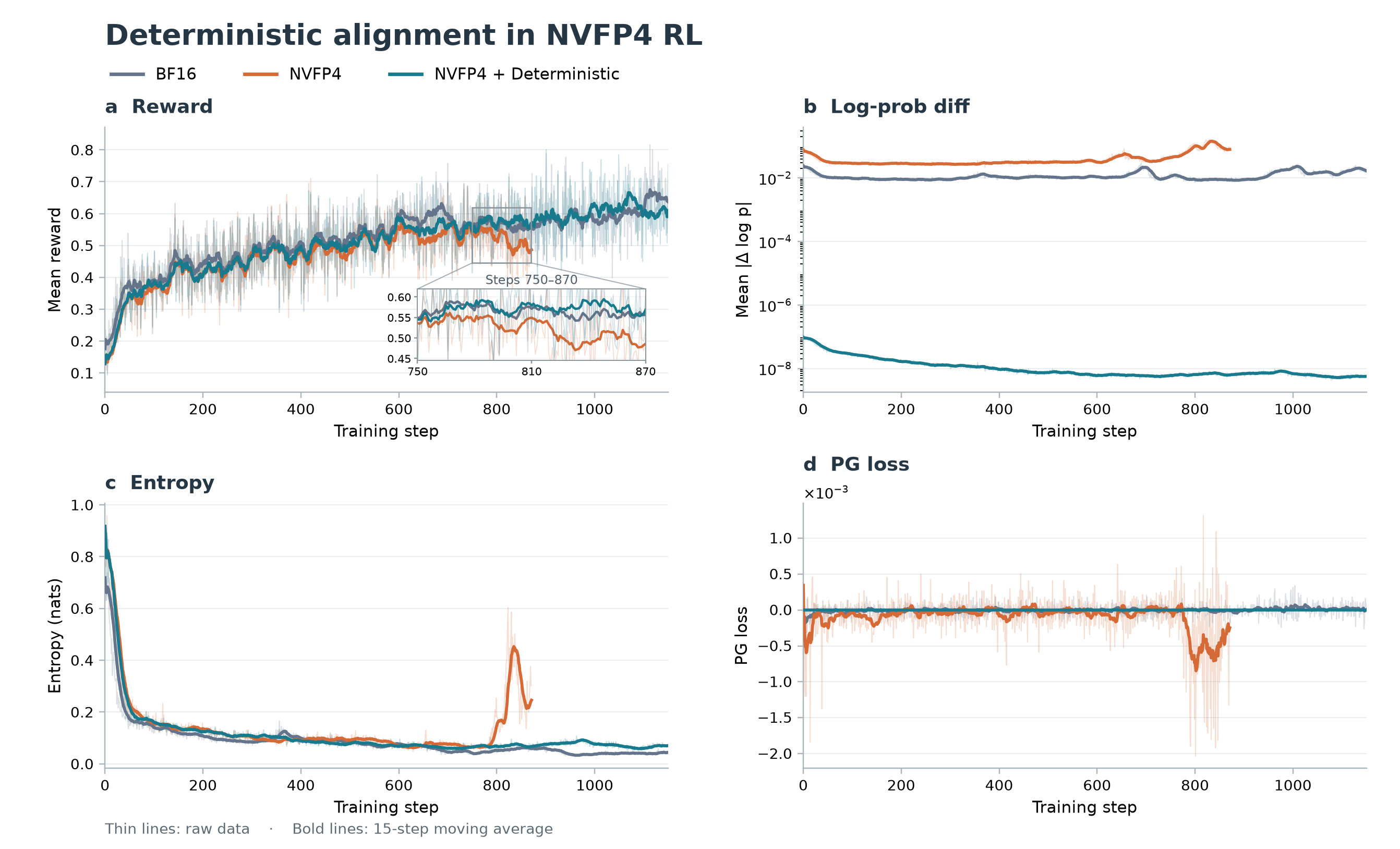
Training dynamics: reward, gap, and entropy follow the training records over steps 0–1199, with endpoints 871/1199/1189. The default is a centered 15-point mean. policy-gradient loss is shown in the four-panel figure below. Strict alignment retains the original joint-intervention configuration.

Open interactive figure: inspect values, switch configurations, download SVG / CSV

Reward, gap, entropy, and policy-gradient loss

Figure 4. Training–sampling alignment: reward, mean absolute log-probability gap, entropy, and policy-gradient loss. Thick lines are 15-step moving averages. The aligned configuration reaches a gap of approximately 10−810^{-8}10−8 over the measured interval and maintains relatively steady late-stage reward. Multiple implementation choices change together in this comparison.

In this experiment, the aligned train–inference log-probability difference falls to approximately 10−810^{-8}10−8, with steady late-stage reward and smaller perturbations. Unaligned NVFP4 shows a late reward decline accompanied by rising entropy and log-probability difference. Within this configuration, smaller train–inference discrepancies accompany steadier NVFP4 RL dynamics. This is a single-run comparison of different implementation configurations with multiple choices changing together. This strict alignment experiment is separate from the practical learning and throughput experiments in Section 6.

miniTE provides alignment capabilities together with the configuration, debugging, and extension interfaces needed to implement them. New low-precision policies can follow the same validation process from local correctness to RL training.

Alignment · §4.5

Under the strictly aligned configuration, the train–inference log-probability gap stays around 10⁻⁸, with stable late-stage reward.

5. Joint NVFP4 Implementation and Optimization with Transformer Engine

5.1 Numerical and Implementation Choices for Per-Token Scaling

We conduct joint testing and implementation work with NVIDIA around TE’s NVFP4 support, using the per-token recipe and its interfaces as an important integration point [9]. Scale granularity affects numerical behavior as well as amax computation, scale storage, and GEMM epilogue cost. Accuracy and speed therefore need to be evaluated together.

NVFP4 encodes data in E2M1, uses an E4M3 scale for each block of 16 elements, and adjusts the range with an outer FP32 scale [1]. Let sis_isi​ be the outer scale of row iii, and bi,jb_{i,j}bi,j​ its length-16 block. Then

di,j=QE4M3 ⁣(amax⁡(bi,j)6si),x^=sidi,jQE2M1 ⁣(xsidi,j).d_{i,j}=Q_{\mathrm{E4M3}}\!\left(\frac{\operatorname{amax}(b_{i,j})}{6s_i}\right), \qquad \hat x=s_i d_{i,j}Q_{\mathrm{E2M1}}\!\left(\frac{x}{s_i d_{i,j}}\right).di,j​=QE4M3​(6si​amax(bi,j​)​),x^=si​di,j​QE2M1​(si​di,j​x​).

Per-tensor scaling shares one outer scale across a tensor; per-token scaling computes it per row. The latter reduces dependence on other tokens’ maxima and can mitigate block-scale underflow when row magnitudes differ greatly. It still retains within-row dynamic-range and FP4 rounding error, and requires finer-grained compute support. Public systems also combine per-token NVFP4 forward computation with higher-precision backward computation [2].

We retain multiple recipes and evaluate numerical choices separately from implementation optimizations. Lower local quantization error alone does not establish more stable RL training. The cost of additional reductions is likewise evaluated over the full computation pa